Introduction
The transition from a planned to a market economy that has been undertaken by the post-communist countries in the EBRD region represents a unique political, social and economic transformation that has taken place in a relatively short period of time. In the last 25 years, the people of those countries have lived through a complete overhaul of their public and social institutions, the emergence of a new private sector, and their reintegration into the global economy. All of those countries suffered an economic recession in the early years of the transition process. In some countries the recession was short-lived, but in others it was deep and lasted many years.
Closing the transition happiness gap
LiTS III data show that there is no longer a gap between post-communist countries and comparators in terms of life satisfaction. Chart 2.1 reports average satisfaction levels for various groups of countries. Countries in Central Asia report very high levels of satisfaction, while central Europe and the Baltic states (CEB) are roughly on a par with Germany and Italy. South-eastern Europe (SEE), eastern Europe and the Caucasus (EEC) and Russia have satisfaction levels similar to those seen in Cyprus, Greece and Turkey.
SOURCE: LiTS III and authors’ calculations.
NOTE: The chart shows the percentage of respondents who agree or strongly agree with the statement “All things considered, I am satisfied with my life now”. The blue bars indicate simple regional averages. The red bars indicate the level of satisfaction when adjusted for individual and household-level characteristics (see Table 2.1). The average for the SEE region does not include Cyprus or Greece, which are shown separately with Turkey.
Life satisfaction and GDP per capita in post-communist and comparator countries
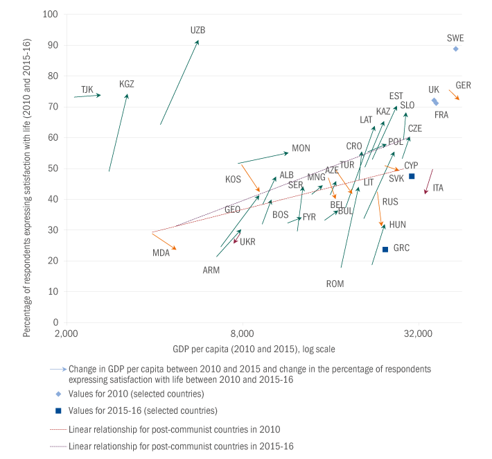
SOURCE: LiTS II and III, World Development Indicators and authors’ calculations.
NOTE: The vertical axis shows the percentage of respondents who agree or strongly agree with the statement “All things considered, I am satisfied with my life now”. The horizontal axis shows GDP per capita in purchasing power parity (PPP) terms (based on 2011 US dollars). Arrows show changes in GDP per capita between 2010 and 2015 and changes in the percentage of respondents expressing satisfaction with their life between 2010 and 2015-16. A green arrow indicates that the country is now better off on both counts, a red arrow indicates that it is worse off on both counts, and a yellow arrow indicates that the country has seen positive income growth but registered a decline in satisfaction levels. The light blue diamonds show GDP per capita in 2010 and the percentage of respondents expressing satisfaction with their life in 2010 for those countries that were surveyed as part of LiTS II only. The blue squares show GDP per capita in 2015 and the percentage of respondents expressing satisfaction with their life in 2015-16 for those countries that were surveyed as part of LiTS III only. The dotted lines show the linear relationships for post-communist countries (excluding the three outliers: the Kyrgyz Republic, Tajikistan and Uzbekistan) in 2010 and 2015-16.
| Satisfied with life (0/1) | |||||||
|---|---|---|---|---|---|---|---|
| (1) | (2) | (3) | (4) | (5) | (6) | (7) | |
| Post-communist country | -0.038 | 0.012 | -0.004 | 0.008 | -0.009 | 0.065 | 0.039 |
| (0.108) | (0.108) | (0.093) | (0.105) | (0.093) | (0.057) | (0.057) | |
| Income | 0.041*** | 0.040*** | 0.041*** | ||||
| (0.007) | (0.007) | (0.007) | |||||
| Can afford holidays and meat | 0.198*** | 0.188*** | 0.190*** | ||||
| (0.016) | (0.016) | (0.014) | |||||
| Can afford unexpected expenses | 0.128*** | 0.121*** | 0.117*** | ||||
| (0.013) | (0.013) | (0.011) | |||||
| Primary education | 0.105*** | 0.046 | 0.107*** | 0.019 | 0.095*** | ||
| (0.034) | (0.130) | (0.034) | (0.121) | (0.027) | |||
| Secondary education | 0.211*** | 0.191 | 0.169*** | 0.160 | 0.157*** | ||
| (0.037) | (0.132) | (0.036) | (0.124) | (0.034) | |||
| Tertiary education | 0.314*** | 0.297** | 0.218*** | 0.262** | 0.205*** | ||
| (0.040) | (0.137) | (0.037) | (0.128) | (0.035) | |||
| Female | 0.026*** | 0.052*** | 0.031*** | 0.042*** | 0.033*** | 0.041*** | 0.030*** |
| (0.006) | (0.009) | (0.006) | (0.009) | (0.006) | (0.009) | (0.005) | |
| Urban area | -0.023** | -0.033** | -0.037*** | -0.045*** | -0.044*** | -0.048*** | -0.049*** |
| (0.011) | (0.016) | (0.011) | (0.015) | (0.011) | (0.016) | (0.012) | |
| Unemployed and looking for a job | -0.188*** | -0.127*** | -0.124*** | -0.118*** | |||
| (0.020) | (0.018) | (0.018) | (0.017) | ||||
| Ethnic minority | 0.003 | 0.002 | -0.005 | 0.014 | 0.002 | 0.009 | 0.000 |
| (0.035) | (0.032) | (0.034) | (0.031) | (0.033) | (0.030) | (0.030) | |
| Number of children | 0.016* | 0.010 | 0.026*** | 0.011 | 0.027*** | 0.011 | 0.028*** |
| (0.009) | (0.007) | (0.009) | (0.007) | (0.008) | (0.007) | (0.008) | |
| Married | 0.034** | 0.044** | 0.023* | 0.042** | 0.022* | 0.042** | 0.020 |
| (0.013) | (0.018) | (0.013) | (0.018) | (0.012) | (0.017) | (0.012) | |
| Divorced or separated | -0.060*** | -0.084*** | -0.046** | -0.081*** | -0.050*** | -0.078*** | -0.049*** |
| (0.019) | (0.024) | (0.017) | (0.025) | (0.017) | (0.024) | (0.017) | |
| Widow or widower | -0.032 | -0.060* | -0.031* | -0.050 | -0.025 | -0.042 | -0.028 |
| (0.020) | (0.032) | (0.017) | (0.032) | (0.018) | (0.031) | (0.017) | |
| Age | -0.009*** | -0.013*** | -0.009*** | -0.013*** | -0.010*** | -0.011*** | -0.010*** |
| (0.002) | (0.003) | (0.002) | (0.003) | (0.002) | (0.003) | (0.002) | |
| Age squared, divided by 100 | 0.008*** | 0.013*** | 0.008*** | 0.013*** | 0.010*** | 0.011*** | 0.009*** |
| (0.002) | (0.003) | (0.002) | (0.003) | (0.002) | (0.003) | (0.002) | |
| No. of observations | 44,551 | 14,715 | 44,551 | 14,715 | 44,551 | 15,956 | 48,963 |
SOURCE: LiTS III and authors’ calculations.
NOTE: This table reports the results of a linear probability model. Standard errors in parentheses are clustered at the country level. *, ** and *** denote values that are statistically significant at the 10, 5 and 1 per cent levels respectively. Income is self-reported in local currency and converted to US dollars and log terms. Dummies for religion (not reported) are statistically significant. Data on the number of children relate to the number of children under the age of 18 who are living at home. Specifications 1 to 5 comprise the 29 post-communist countries plus Germany and Italy. Specifications 6 and 7 also include Cyprus, Greece and Turkey.
Lasting impact of the early years of the transition process
Chart 2.3 shows the evolution of average height in post-communist countries as a function of the difference between respondents’ birth year and the year when transition occurred. Average height gradually increased over time, before declining in cohorts born two to three years before transition occurred and remaining depressed for a number of years. The first sustained increases in average height were observed in cohorts born six years after transition, at which point average height returned to the pre-transition trend level. Differences in height between people born around the time of the transition process and the trend are statistically significant.
SOURCE: LiTS III and authors’ calculations.
NOTE: The line denotes average height in post-communist countries, calculated as a three-year moving average. The horizontal axis shows the difference between the respondent’s year of birth and the year when transition occurred (with the transition year varying from country to country, as Box 2.1 explains).
SOURCE: Gapminder, LiTS III and authors’ calculations.
NOTE: The blue diamonds show average height by birth year, calculated as a three-year moving average, while the green line shows a population-weighted three-year moving average of GDP per capita. Averages are calculated for four comparator countries: Cyprus, Germany, Greece and Italy. GDP per capita is expressed in PPP terms (based on 2011 US dollars).
| (1) | (2) | (3) | (4) | |
|---|---|---|---|---|
| Born in transition year | Born or one year old in transition year | Born in transition year | Born or one year old in transition year | |
| Born in transition | -1.057*** | -0.768*** | -0.777* | -0.544* |
| (0.398) | (0.282) | (0.409) | (0.292) | |
| Average of log GDP per capita | 1.129*** | 1.190*** | ||
| (0.215) | (0.221) | |||
| No. of observations | 42,853 | 42,853 | 40,854 | 40,887 |
| R2 | 0.382 | 0.382 | 0.384 | 0.384 |
SOURCE: LiTS III, Correlates of War Data, EBRD transition indicators, Gapminder, UCDP/PRIO Armed Conflict Dataset, and authors’ calculations.
NOTE: Standard errors in parentheses are clustered at the PSU level. *, ** and *** denote values that are statistically significant at the 10, 5 and 1 per cent levels respectively. All specifications control for country fixed effects and country-specific linear time trends. In addition, the gender of the respondent, whether the respondent was born in an urban or rural location, the respondent’s religion, the parents’ level of education and the incidence of war are also included as controls. Specifications 3 and 4 also control for the parents’ employment sector and the log of GDP per capita.
| (1) | (2) | (3) | (4) | |
|---|---|---|---|---|
| Born in transition year | Born or one year old in transition year | Born in transition year | Born or one year old in transition year | |
| Change in price liberalisation indicator | -0.565*** | -0.343*** | -0.466** | -0.274** |
| (0.194) | (0.114) | (0.204) | (0.119) | |
| Average of log GDP per capita | 1.267*** | 1.323*** | ||
| (0.229) | (0.233) | |||
| No. of observations | 36,507 | 36,507 | 34,660 | 34,693 |
| R2 | 0.373 | 0.373 | 0.375 | 0.375 |
SOURCE: LiTS III, Correlates of War Data, EBRD transition indicators, Gapminder, UCDP/PRIO Armed Conflict Dataset, and authors’ calculations.
NOTE: Standard errors in parentheses are clustered at the PSU level. *, ** and *** denote values that are statistically significant at the 10, 5 and 1 per cent levels respectively. All specifications control for country fixed effects and country-specific linear time trends. In addition, the gender of the respondent, whether the respondent was born in an urban or rural location, the respondent’s religion, the parents’ level of education and the incidence of war are also included as controls. Specifications 3 and 4 also control for the parents’ employment sector and the log of GDP per capita.
| Satisfied with life (0/1) | Satisfaction with life (1-5) | |||
|---|---|---|---|---|
| (1) Born in transition year |
(2) Born or one year old in transition year |
(3) Born in transition year |
(4) Born or one year old in transition year |
|
| Born in transition | 0.141* | 0.104* | 0.148*** | 0.094** |
| (0.079) | (0.056) | (0.057) | (0.041) | |
| No. of observations | 47,059 | 47,059 | 47,059 | 47,059 |
SOURCE: LiTS III, Correlates of War Data, EBRD transition indicators, UCDP/PRIO Armed Conflict Dataset, and authors’ calculations.
NOTE: Standard errors in parentheses are clustered at the PSU level. *, ** and *** denote values that are statistically significant at the 10, 5 and 1 per cent levels respectively. All specifications control for country fixed effects and birth year fixed effects. In addition, the gender of the respondent, whether the respondent was born in an urban or rural location, the respondent’s religion, the parents’ level of education and the incidence of war are also included as controls.
| (1) Satisfied with life (0/1) |
(2) Preference for a market economy |
(3) Preference for democracy |
(4) Preference for redistribution |
(5) Trust |
|
|---|---|---|---|---|---|
| Experience of transition in formative years | -0.019 | 0.026* | 0.026* | 0.040 | 0.039 |
| (0.014) | (0.014) | (0.014) | (0.084) | (0.029) | |
| No. of observations | 42,489 | 37,927 | 39,280 | 41,676 | 41,599 |
SOURCE: LiTS III, Correlates of War Data, EBRD transition indicators, UCDP/PRIO Armed Conflict Dataset, and authors’ calculations.
NOTE: Standard errors in parentheses are clustered at the PSU level. *, ** and *** denote values that are statistically significant at the 10, 5 and 1 per cent levels respectively. All specifications control for country fixed effects and birth year fixed effects. In addition, the respondent’s gender, whether the respondent was born in an urban or rural location, the respondent’s religion, the parents’ level of education and the incidence of war are also included as controls.
Heterogeneity in the impact of transition
The impact of transition has not been equally distributed across society. This section documents the ways in which the transition process has affected different social groups. Not surprisingly, the most vulnerable people have been those born to disadvantaged families.
There are no data on the living standards of the parents of LiTS respondents prior to the transition process. Consequently, for the purposes of the analysis in this section, those living standards are proxied by parental labour force participation and parents’ level of education. In this section, the impact that the transition process has had on well-being is estimated separately for subsamples with different parental backgrounds. In particular, Chart 2.5 reports the impact that transition has had on satisfaction on the basis of the mother’s labour force participation. As was shown in the previous section, cohorts who were born or turned one in the transition year are, on average, actually happier than their peers. However, this is not the case where the respondent’s mother has never worked. On the contrary, those respondents appear to be less satisfied with their lives as a consequence of being born at that time. Such families account for around 20 per cent of the sample.
SOURCE: LiTS III, Correlates of War Data, EBRD transition indicators, Gapminder, UCDP/PRIO Armed Conflict Dataset, and authors’ calculations.
NOTE: The dark grey bars show the sum of the coefficients for the “born in transition” indicator and the interaction term (signalling that the mother has never worked) and indicate the impact that transition has had on those respondents whose mothers have never participated in the labour market. The blue bars show the coefficient for the “born in transition” indicator and indicate the impact that transition has had on those respondents whose mothers have participated in the labour market at some point in their life. These effects are calculated after controlling for individual and parental characteristics.
SOURCE: LiTS III, Correlates of War Data, EBRD transition indicators, Gapminder, UCDP/PRIO Armed Conflict Dataset, and authors’ calculations.
NOTE: The bars show the sum of the coefficients of the “born in transition” indicator and the interaction term (indicating the mother’s level of education). These effects are calculated after controlling for individual and parental characteristics.
SOURCE: LiTS III, Correlates of War Data, EBRD transition indicators, Gapminder, UCDP/PRIO Armed Conflict Dataset, and authors’ calculations.
NOTE: The bars show the sum of the coefficients for the “born in transition” indicator and the interaction term (indicating the mother’s level of education). These effects are calculated after controlling for individual and parental characteristics.
Ruling out alternative explanations
Could the results detailed above be driven by other events that coincided with the transition process? The transition period was preceded by various highly consequential political and economic developments – primarily the fall of the Berlin Wall and the dissolution of the Soviet Union – which marked the end of an era and heralded the beginning of a new order. In order to rule out the possibility that the results set out in this chapter were driven by those events, a set of placebo tests have been run to ensure that people who were born or in their infancy in the two years in question (namely, 1989 and 1991 respectively) do not differ from their younger and older peers in terms of height or satisfaction. The results of those tests show that those events do not explain the main findings of this chapter, demonstrating that it really is exposure to the transition process (which began at different times in different countries) – and not simply being born around the time of the fall of the Berlin Wall or the dissolution of the Soviet Union – that has caused respondents in post-communist countries to be shorter than their peers.
Conclusion
This chapter uses a unique Life in Transition Survey to measure the impact that transition from a planned to a market economy has had on well-being. In the past, research has found people in post-communist countries to be less happy than peers in countries that have not experienced such a transition (even after controlling for income), with some researchers suggesting that this “transition happiness gap” represents a temporary phenomenon that will eventually disappear. LiTS III, which surveyed more than 51,000 households in 29 post-communist countries and five comparator countries, confirms that this gap has finally been closed: when income is controlled for, residents of post-communist countries no longer lag behind their counterparts in terms of reported levels of satisfaction.
However, this does not mean that the pain of the transition process was not real. LiTS III provides information that helps to quantify the magnitude of the socio-economic shock that was experienced in the first few years of the transition process. Comparing the height of individuals experiencing transition in their first two years of life, this chapter finds that those individuals are, on average, around 1 cm shorter than their younger and older peers. This confirms the view that the first few years of the transition process were a period of substantial socio-economic deprivation. At the same time, that shock does not seem to have had negative long-term implications for those individuals’ levels of satisfaction or attitudes. If anything, cohorts born around the time of the transition process are now happier (and better educated) than their peers.
The other important finding in this chapter is that, while the process of “happiness convergence” has, on the whole, been completed, certain sections of society still lag behind. Not surprisingly, this concerns individuals born to families with low levels of maternal education and employment (who make up 20 per cent of the cohorts born around the time of the transition process).
This analysis of the impact that transition has had on well-being has important implications not only for the few remaining command economies around the world, but also, more generally, for countries undertaking major structural reforms. First of all, it is important that happiness convergence has finally been achieved. In this respect, economic reforms – despite being incomplete in some countries – have eventually delivered (albeit much later than was initially expected). Second, the fact that it has taken these post-communist countries 25 years to catch up with their peers in terms of happiness should not discourage reformers elsewhere. Even major reforms to labour markets and pension systems are less disruptive – and, therefore, arguably less painful – than the systemic changes that these post-communist countries have gone through. Third, lessons learned from previous reforms can help to make such initiatives less painful and more inclusive in the future. Potential losers in such reform processes should be given not only one-off compensation, but also the skills necessary to ensure their future employability. Unfortunately, the complexity of such reforms, the large number of stakeholders involved and the dynamic nature of the interaction between them mean that the identification of potential losers is highly context-specific.16
Lastly, this chapter’s optimistic overall message also points to a major risk relating to the “short-term pain, long-term gain” scenario. The risk here is that the political reaction to the pain of reforms could persist even after the pain has gone. Although the effects of the initial transition shock in post-communist countries can no longer be seen at the level of households, some countries have experienced policy reversals that persist to this day. That transition shock has armed opportunistic politicians with an anti-reform narrative, which has ultimately resulted in de-democratisation.17 Where these politicians have gained power, they have gone on to undermine both democratic political institutions and economic institutions.18 The subsequent removal of democratic checks and balances has now made it hard to vote these politicians out of office, despite their original anti-transition platform having ceased to be valid. In order to avoid such lasting political implications, reformers should try to compensate potential losers in reform processes from the outset, preventing populists from potentially destroying political institutions.
Box 2.1. Methodology used to analyse the impact on well-being
This chapter analyses the impact that the transition process has had on objective and subjective well-being at the level of individual respondents. The primary data source for this chapter is the third round of the Life in Transition Survey, which was conducted by the EBRD and the World Bank in 34 countries in late 2015 and the first half of 2016. The results of that survey will be published later this year. A total of 75 locations were visited in each of the countries surveyed, with more than 51,000 interviews being conducted with randomly selected households.
The main variables that are of interest for the analysis presented here are (self-reported) height and life satisfaction.19 The latter is captured in two ways: using a binary variable that simply indicates whether or not the respondent agrees or strongly agrees with the statement “All things considered, I am satisfied with my life now”; and using a continuous variable with a five-point scale. LiTS III also provides data on respondents’ support for democracy and the market economy, optimism,20 preferences regarding income redistribution, generalised social trust and active membership of associations.
The chapter begins with analysis of the transition happiness gap, which is based on the conventional econometric model of satisfaction:

where the binary dependent variable for individual i, born in country c and aged ![]() , is regressed on an indicator that takes a value of 1 if c is a post-communist country, as well as a vector of individual characteristics (
, is regressed on an indicator that takes a value of 1 if c is a post-communist country, as well as a vector of individual characteristics (![]() ) listed in Table 2.1. These include age and age squared (or, alternatively, birth year fixed effects). Standard errors
) listed in Table 2.1. These include age and age squared (or, alternatively, birth year fixed effects). Standard errors ![]() are clustered at the country level.
are clustered at the country level.
The coefficient ![]() denotes the effect that living in a post-communist country has on life satisfaction (when controlling for conventional individual and household-level determinants of happiness). If
denotes the effect that living in a post-communist country has on life satisfaction (when controlling for conventional individual and household-level determinants of happiness). If ![]() is negative and significant, this means that the transition happiness gap is still present; if there is no significant negative effect, the gap has been closed.
is negative and significant, this means that the transition happiness gap is still present; if there is no significant negative effect, the gap has been closed.
The second part of the chapter looks at the way in which the effect of the transition process varies depending on when people were born. First, it evaluates the physical impact of the transition process by comparing anthropometric indicators for people who were born or turned one or two during transition with those of individuals who were born before or after that period.21 Although the environment where a person grows up determines only around 20 per cent of adult height, it accounts for most of the cross-population variation in that indicator.22 Final adult height depends crucially on the speed of growth during the first two years of life – which, in turn, depends on living standards in the household during that period. A similar analysis is repeated for the life satisfaction of cohorts who were born or turned one or two during transition.
It then assesses the impact that the transition process has had on people’s attitudes and life satisfaction. This analysis is based on the assumption that individual beliefs and attitudes are shaped in a person’s formative years, which are defined as the period between the ages of 18 and 25 and broadly correspond to the moment when individuals enter the labour market for the first time.23 Interdisciplinary research provides evidence of the importance of this stage in life as regards the formation of political and interpersonal attitudes.24
For the purposes of the statistical analysis in this chapter, the transition period is defined as the year when the country in question made significant progress with price liberalisation reforms (which corresponds to the point at which the EBRD’s price liberalisation indicator for that country reached a value of 3 for the first time). Overall, 12 countries implemented the bulk of their price liberalisation reforms between the fall of the Berlin Wall and the dissolution of the Soviet Union, and 12 other countries followed suit between 1992 and 1993. The five remaining countries did not implement reforms until later, doing so between 1994 and 1995.
This analysis also includes alternative continuous measures of transition tracking ongoing progress with reforms – namely, changes in the EBRD’s price liberalisation indicator and changes in the average of all six transition indicators over a given period of time.25 As with the approach described above, three variables are created, indicating (i) the change in the respondent’s year of birth relative to the previous year, (ii) the change in the year when the respondent turned one relative to the year before his/her birth, and (iii) the change in the year when the respondent turned two relative to the year before his/her birth. For the analysis of formative years, changes are calculated for the period when the respondent was 18 to 25 years old.
These binary and continuous measures of reform should not be seen as substitutes, but rather as complements, since they assess different facets of the transition process and address critical concerns regarding the causality of the analysis. Indeed, a major challenge for the analysis is the question of reverse causality. In planned economies that were bankrupt and experiencing severe shortages of vital nutrients before reforms took place, political and economic transition might, in fact, have been a consequence of deprivation, rather than the other way round. Controlling for fluctuations in GDP and using continuous variables indicating changes in the price liberalisation indicator or the average of all transition indicators should address these concerns.
This chapter’s analysis of the impact that the transition process has had on height is based mainly on the following specification:

where the reported height of individual i, born in year y and country c, is regressed on an indicator – “born in transition” – which takes a value of 1 if the individual was born or turned one in the year when transition occurred. ![]() is a vector of individual and household-level characteristics, as well as country-specific factors, all of which are likely to affect the outcomes of interest. These controls include gender, whether the respondent was born in an urban or rural location, religion and parental background (namely, parents’ level of education and employment sector). At the country level, regressions control for GDP per capita and incidence of war.26 Country fixed effects (
is a vector of individual and household-level characteristics, as well as country-specific factors, all of which are likely to affect the outcomes of interest. These controls include gender, whether the respondent was born in an urban or rural location, religion and parental background (namely, parents’ level of education and employment sector). At the country level, regressions control for GDP per capita and incidence of war.26 Country fixed effects (![]() ) capture any time-invariant country characteristics, while country-specific linear time trends control for the natural increases in height that are typically seen over time in most middle-income countries. The country-specific linear trend is defined as follows:
) capture any time-invariant country characteristics, while country-specific linear time trends control for the natural increases in height that are typically seen over time in most middle-income countries. The country-specific linear trend is defined as follows: The same specification is used for the continuous measures of reform discussed above. The “born in transition” indicator is replaced with the change in the price liberalisation indicator or the change in the average of all six transition indicators over the relevant period of time.
The analysis of the impact on attitudes and satisfaction with life uses a third specification:

where the outcome (satisfaction with life, trust, and attitudes to the market economy, democracy, redistribution and so on) is regressed on the “born in transition” indicator, as well as ![]() – a vector of controls including gender, whether the respondent was born in an urban or rural location, religion, parents’ level of education and incidence of war. Country fixed effects (
– a vector of controls including gender, whether the respondent was born in an urban or rural location, religion, parents’ level of education and incidence of war. Country fixed effects (![]() ) and birth year fixed effects (
) and birth year fixed effects (![]() ) are also included.
) are also included.
Birth year fixed effects control for highly non-linear relationships between age and life satisfaction, while the regressions can still identify the effects of being “born in transition” because countries are considered to have undergone transition in different years. A 25-year-old living in a country where transition took place in 1990 is classified as having been born after transition (if the survey was conducted in 2016). However, a person of the same age living in a country where transition took place in 1993 is considered to have been born two years before the start of transition, so his/her height and satisfaction with life are likely to have been affected by that process.
As above, the same specification is used to repeat this analysis using the continuous measures of reform. Lastly, the same specification is also used to analyse the impact on the attitudes and satisfaction levels of people who were aged 18 between 25 when the transition process occurred.27
Box 2.2. Analysis of the impact of transition on well-being in Russian panel data
The results derived from the Life in Transition Survey can be validated by another household survey – the Russian Longitudinal Monitoring Survey (RLMS) conducted by the Higher School of Economics in Moscow. Although the RLMS covers only one country, it has two unique advantages. Its panel dataset consists of various survey rounds from 1994 to 2014, including both adult and child respondents from individual households, which means that the impact that transition has had on children’s heights can be measured while controlling for the height of parents.28 It also allows within-family analysis, making it possible to see the effect of being born during transition by comparing a child with a sibling who was born before or after transition took place.
| Adults (cm) | Children (height-for-age z-scores) | Children – within-family (height-for-age z-scores)29 | ||||
|---|---|---|---|---|---|---|
| (1) | (2) | (3) | (4) | (5) | (6) | |
| Born in transition year | Born or one year old in transition year | Born in transition year | Born or one year old in transition year | Born in transition year | Born or one year old in transition year | |
| Born in transition | -1.392*** | -1.514*** | -0.216** | -0.221*** | -0.545** | -0.449** |
| (0.382) | (0.286) | (0.100) | (0.080) | (0.257) | (0.191) | |
| Implied change in adult height – girls (cm) | -1.47 | -1.5 | -3.71 | -3.05 | ||
| Implied change in adult height – boys (cm) | -1.56 | -1.59 | -3.92 | -3.23 | ||
| No. of observations | 39,736 | 39,736 | 10,552 | 10,552 | 3,106 | 3,106 |
| R2 | 0.514 | 0.514 | 0.154 | 0.155 | 0.571 | 0.571 |
SOURCE: RLMS, EBRD transition indicators, and authors’ calculations.
NOTE: Standard errors are shown in parentheses. *, ** and *** denote values that are statistically significant at the 10, 5 and 1 per cent levels respectively. All specifications control for the respondent’s gender and whether he/she is resident in an urban location, as well as regional linear trends and region fixed effects. Specifications 3 and 4 also control for the mother’s level of education and height, while specifications 5 and 6 control for family fixed effects. In specifications 1 to 4, standard errors are clustered by region. Within-family estimates (specifications 5 and 6) only include data derived from surveys between 1994 and 2008 in the interests of consistency regarding family identifiers. Children’s heights are converted into height-for-age z-scores after subtracting the average and dividing by the standard deviation of the heights of US children of the same age in the WHO Global Database based on US population data.
References
D. Almond (2006)
“Is the 1918 Influenza Pandemic Over? Long-Term Effects of In Utero Influenza Exposure in the Post-1940 U.S. Population”, Journal of Political Economy, Vol. 114(4), pp. 672-712.
A. Beard and M. Blaser (2002)
“The Ecology of Height: The Effect of Microbial Transmission on Human Height”, Perspectives in Biology and Medicine, Vol. 45(4), pp. 475-498.
A. Case (2004)
“Does Money Protect Health Status? Evidence from South African Pensions”, in D. Wise (ed.), Perspectives on the Economics of Aging, pp. 287-312.
A. Case and C. Paxson (2010)
“Causes and Consequences of Early-Life Health”, Demography, supplement to Vol. 47(1), pp. S65-S85.
A. Deaton (2008)
“Income, Health, and Well-Being around the World: Evidence from the Gallup World Poll”, Journal of Economic Perspectives, Vol. 22(2), pp. 53-72.
S. Djankov (2016)
“The Divergent Post-Communist Paths to Democracy”, Journal of Economic Perspectives, forthcoming.
S. Djankov, E. Nikolova and J. Zilinsky (2016)
“The Happiness Gap in Eastern Europe”, Journal of Comparative Economics, Vol. 44(1), pp. 108-124.
E. Duflo (2003)
“Grandmothers and Granddaughters: Old-Age Pensions and Intrahousehold Allocation in South Africa”, World Bank Economic Review, Vol. 17(1), pp. 1-25.
R. Easterlin (2014)
“Life Satisfaction in the Transition from Socialism to Capitalism”, in A. Clark and C. Senik (eds.), Happiness and Economic Growth: Lessons from Developing Countries, pp. 6-31.
EBRD (2013)
Transition Report 2013: Stuck in Transition?, Chapter 3, London.
P. Giuliano and A. Spilimbergo (2014)
“Growing up in a Recession”, Review of Economic Studies, Vol. 81, pp. 787-817.
N. Gleditsch, P. Wallensteen, M. Eriksson, M. Sollenberg and H. Strand (2002)
“Armed Conflict 1946-2001: A New Dataset”, Journal of Peace Research, Vol. 39(5), pp. 615-637.
S. Guriev and E. Zhuravskaya (2009)
“(Un)happiness in Transition”, Journal of Economic Perspectives, Vol. 23(2), pp. 143-168.
P. Kozyreva, M. Kosolapov and B. Popkin (2016)
“Data Resource Profile: The Russia Longitudinal Monitoring Survey—Higher School of Economics (RLMS-HSE) Phase II: Monitoring the economic and health situation in Russia, 1994–2013”, International Journal of Epidemiology, Vol. 45(2), pp. 395-401.
L. Li, O. Manor and C. Power (2004)
“Early Environment and Child-to-Adult Growth Trajectories in the 1958 British Birth Cohort”, The American Journal of Clinical Nutrition, Vol. 80(1), pp. 185-192.
NCD Risk Factor Collaboration (2016)
“A century of trends in adult human height”, eLife, Vol. 5.
M. Nikolova (2016)
“Minding the Happiness Gap: Political Institutions and Perceived Quality of Life in Transition”, European Journal of Political Economy, forthcoming.
N. Persico, A. Postlewaite and D. Silverman (2004)
“The Effect of Adolescent Experience on Labor Market Outcomes: The Case of Height”, Journal of Political Economy, Vol. 112(5), pp. 1019-1053.
T. Pettersson and P. Wallensteen (2016)
“Armed Conflicts, 1946-2014”, Journal of Peace Research, Vol. 52(4), pp. 536–550.
G. Roland (2014)
“Transition in Historical Perspective”, in A. Aslund and S. Djankov (eds.), The Great Rebirth: Lessons from the Victory of Capitalism Over Communism, Peterson Institute for International Economics.
P. Saenger, P. Czernichow, I. Hughes and E. Reiter (2007)
“Small for gestational age: short stature and beyond”, Endocrine Reviews, Vol. 28, pp. 219-251.
P. Sanfey and U. Teksoz (2007)
“Does Transition Make You Happy?”, Economics of Transition, Vol. 15(4), pp. 707-731.
M. Sarkees and F. Wayman (2010)
“Resort to war: A data guide to inter-state, extra-state, intra-state, and non-state wars, 1816-2007”, CQ Press, Washington, D.C.
R. Steckel (1995)
“Stature and the Standard of Living”, Journal of Economic Literature, Vol. 33, pp. 1903-1940.
B. Stevenson and J. Wolfers (2008)
“Economic Growth and Subjective Well-Being: Reassessing the Easterlin Paradox”, Brookings Papers on Economic Activity, Vol. 39(1), pp. 1-102.
D. Treisman (2014)
“The Political Economy of Change After Communism”, in A. Aslund and S. Djankov (eds.), The Great Rebirth: Lessons from the Victory of Capitalism Over Communism, Peterson Institute for International Economics.